Extracting Stable Behavior from Learned Policy

  The hidden-state reinforcement learning procedure described above can learn to solve active recognition problems. However, as is true with all reinforcement learning approaches it can take considerable exploration to find the optimal solution. Since we use a memory based approach, storing all previous experience, this has the disadvantage that the learned representation can grow quite large. (And keeps on growing, if the algorithm is implemented literally.)

We ran experiments to measure the amount of experience and random search needed by the hidden-state reinforcement learning system to find active recognition policies in the interactive interface domain. In each experiment we ran the learning system with a random user state to be the target, and used the remaining states in $\cal W$to be distractors. While correct performance was eventually achieved in each case, it can take a considerable number of steps to find a solution. Averaged over 22 experiment trials, there were approximately T=2973 experience time-steps in the system before a solution was found, even though the most complicated recovered recognition strategy contained no more than four actions! This is not entirely unsurprising, since the system needs to average reward across many trials to avoid perceptual aliasing, and perform considerable random exploration to find solutions.

A typical solution executes a small number of actions in only few different perceptual conditions. I.e., to detect a target gesture where the user is smiling and pointing with her right hand, the system waits until it sees a form with extended arm, then looks to the face, if it sees a smile expression it then looks to the right-hand, and then if it sees a point gesture it generates the accept action. Since the actual behavior of the algorithm after convergence can be quite simple, it seems desirable to attempt to capture just this simple behavior, and eliminate experience not needed for its performance.

A further problem is that the Q-learning policy is sensitive to the distribution of target vs. non-target trials. In Q-learning the utility of actions is constantly updated; if the target stops appearing, or if the distractors which are perceptually aliased with the target stop appearing, then the system will evolve towards a new policy which is optimal to the distribution of targets at the current moment, but may not be the desired policy. This plasticity is of course the central feature of general learning methods, but at some point we may wish to fix utilities and remove this dependence. We may need to have a statistically representative training set during learning, but it is desirable to have no such requirements for the testing set.

Our innovation to overcome these problems is to devise a method for extracting a visual behavior-like representation from the learned policy. We observe that after convergence of the learning algorithm, the utility values represent the average expected reward propagated backwards through time and discounted appropriately, (i.e. a time-discounted approximation to the confidence that we will detect the target). We thus no longer need the actual experience containing the raw rewards, if we can extract or reconstruct the relevant representation of utility. We further observe that the experience representation used in our hidden-state reinforcement learning method shares certain similarities to a representation that is simply a series of state transitions, with links augmented with actions as well as observation pre-conditions. Indeed, we can transform our learned policy into a state transition representation, and eventually into a Finite State Machine augmented with action transition labels.

Conversion to an augmented Finite State Machine (aFSM) has several advantages for representing run-time recognition behavior. It is more stable, compact, and does not require any of the matching or learning machinery presented in the previous section. Indeed, the states that are implicitly represented in the instance-based method are made explicit in the aFSM representation. The aFSM is defined by a set of recognition states $\cal RS$ and a set of directed links $\cal L$ each labeled with an associated observation and action pair. Terminal nodes are labeled with target identity, and transition into them indicate detection of the target. We use three steps to convert our reinforcement policy to aFSM: utility space pruning, conversion to a recognition state chain, and finally integration of multiple target strategies. We will discuss each of these in turn. We also will show how recognition policies learned for multiple targets can be merged during conversion to the aFSM representation.

 

Figure 4:   Active recognition policy used in hidden-state reinforcement learning method, after pruning algorithm described in Section 4.1 is applied.

 

Figure 5:   Augmented Finite State Machine representation of three different active recognition policies. Circles indicate state, arcs are labeled transitions marked with ``o|a'', where o is the list of observations that are a precondition for link traversal, and a is an action to execute when traversing the link. Dashed lines inidicate the default traversal when no precondition is met. An asterisk marks the initial state, and the shaded circle marks the terminal state indicating recognition. (a) recognizes the gesture where the user is smiling and pointing with his right hand with his left arm down, (b) the gesture where the user is smiling, pointing with the right hand, and has his left hand open, and (c) the gesture where the user is smiling, has the right hand open and is pointing with his left hand.

 

Figure 6:   Initial stage of merging the three different recognition strategies presented in previous figure. Terminal nodes are marked with object / gesture identity.

 

Figure 7:   Final active recognition aFSM after duplicate preconditions have been eliminated from the aFSM in the previous figure, using algorithm described in Section 4.3.

Run-time action-selection and utility-space pruning

  We first note that once correct behavior has been learned, the utility values contain all the relevant information for action selection at run-time. I.e., the selection of new actions in Equations (6,5) depends only on q[i], and not on r[i]. Rewards only have influence in the Q-learning update step, Equation (8). Thus when the utility values have converged to optimal behavior for a given target and distribution of distractors, we no longer need to perform this update step; this renders the reward values themselves no longer of use, and freezes the utility value space. This has the immediate potential benefit that the system will now behave independent of the future distribution of targets and distractors.

For many if not most recognition tasks, a small subset of the learned utility space is sufficient to drive successful recognition. Since the null action is always available at zero utility or greater, regions of the utility space with negative utility will, as can be seen in Equation (6), never influence action selection. We can thus set to zero any negative utility values, and further prune the memory of any experience tuple with zero utility assuming the observation and action of that experience are never used in the nearest sequence matching process when a positive utility value is returned.

Most powerfully, we observe that after utility space convergence, recognition behavior for our task can be driven solely from utility associated with experience with the target. When utility values have properly converged the representation of regions of utility space defined only by experiences with distractors is irrelevant: any instances of positive utility values in distractor trials will occur over subsequences of experience that are perceptually aliased with target trials, and the copy of those experiences in the target trials is sufficent to drive correct recognition behavior.

Our final experience pruning observation is that any target trials which are redundant due to equivalent observation and action sequences can be merged together without affecting action selection. Based on these observations, we perform the following steps to prune the action-selection policy computed from reinforcement learning once the policy has converged to correct performance:

• Utility values are frozen; the Q-learning update step (Equation 8) is no longer applied.
• Execution continues for fixed number of trials (sufficient such that several experiences with the target pattern will be observed), discarding any new trial which either has uniformly negative utility or which is known to be a distractor trial.
• The memory of all trials collected prior to pruning is discarded, retaining only those trials collected while learning was frozen.
• Any two trials which have equivalent observation and action sequences are merged.

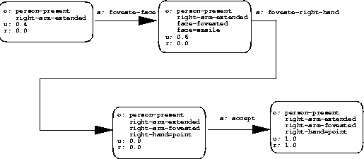
We have found that this pruning method can extract representations of utility that capture recognition behavior for our tasks in an intuitive and efficient way. Typically, one or two chains are recovered, which simply list the steps required to discriminate target from distractor. Figure 4 shows the memory-based action selection policy for one of the randomly selected targets in the experiment described above. The solution to these recognition problems generally involves first checking to see if the coarse pose is the same as the target, then observing the face; if the face pose matches the target then one or both hands is observed. If all hidden features match the target, accept is generated.

Conversion to recognition-state chain

To convert from hidden-state action-selection policy to an aFSM representation, we first compute a set of recognition states $\cal RS$ corresponding to the implicit states of the active recognition system expressed in the learned policy. Recall that the nearest sequence matching algorithm associates utility with sequences of action/observation tuples of varying length, so each subsequence of a recovered experience chain is a possible recognition state.

The set of actual recognition states used by a particular policy is found by marking the ``nearest neighbor'' sequences which lead to computation of positive utility in Equation 5 when the pruned policy is executing. I.e., whenever a positive utility value is returned by Equation 5, for each voting time-step v[i] we define a recognition state to be associated with the M(i-1,T) previous time-steps (recall M(i-1,T) is the match length associated with v[i]).

Each recognition state will thus correspond to an action/observation sequence of varying length in the learned policy. We look in the policy to determine what transitions are defined between recognition states. For each recognition state whose policy sequence ``follows'' another recognition state we note the action and observation linking the two, and add a link to $\cal L$ (the set of labeled links in the aFSM). Each link is labeled with the observation as a precondition of traversal, and the action to take when traversing the link. ``Follows'' here is defined to mean that the endpoint of the subsequence corresponding to one recognition state is one time-step earlier than the endpoint of the subsequence corresponding to the following recognition state.

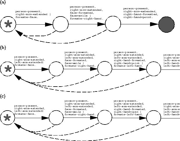
For the example in Figure 4, three recognition states are found, not surprisingly corresponding to the progressive revelation of the hidden features of the target pattern. Figure 5(a) shows the recognition state chain corresponding to this example.

Integration of multiple target strategies

  Finally we convert the recognition state chain into an aFSM. We add default links returning the system to the initial state when no perceptual condition is satisfied, and we define recognition states entered following the accept action to be terminals.

It is also straightforward to integrate strategies for recognizing different targets at this point. We separately train policies corresponding to different target patterns, and then use syntactic heuristics to merge them at the recognition state level. Equivalent recognition states in each chain (or aFSM) are merged, taking the union of links to subsequent states. We also merge the initial states from each separate aFSM.

When merging states, we check to see whether duplicate perceptual conditions are present for any recognition state, and if so we re-arrange the links appropriately. If two links l₁, l₂ exiting state s₀ leading to new states s₁,s₂ have the same observation precondition, and they have the same action a₁,a₂, we delete l₂, and merge s₁ with s₂. If a₁ and a₂ are different, we set the default action from s₁ to point to s₂, and label it with the action on l₂. (If s₁ already had a labeled default action, we follow this default action link forward iteratively until we come to a state with an unlabeled default action, and then set it to point to s₂ with the action on l₂.)

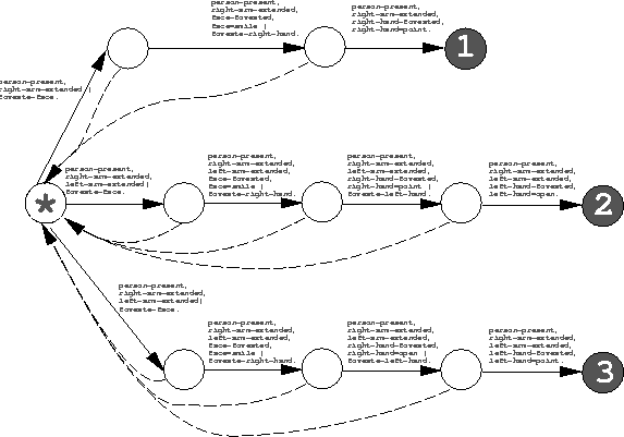
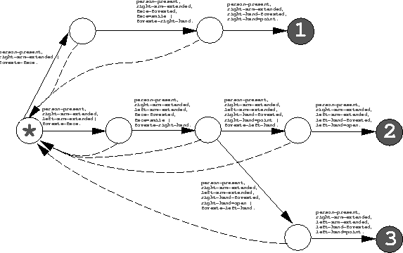
Figure 5 shows three recognition state chains found for different targets in our example. Simply connecting together the initial state of these three chains yields the (invalid) aFSM shown in Figure 6. The initial state has links with common observation precondition; we remove them as described above, yielding the final (correct) aFSM recognition behavior shown in Figure 7. This aFSM will direct foveation to detect any of its three target patterns when present, and will not be confused by any other possible user configuration.