CS 184: COMPUTER GRAPHICS
Heads-up!! -- Midterm-Exam: in class on Wednesday 3/16 -- be prepared; show up on time!
How to prepare for the Midterm-Exam
PREVIOUS
< - - - - > CS
184 HOME < - - - - > CURRENT
< - - - - > NEXT
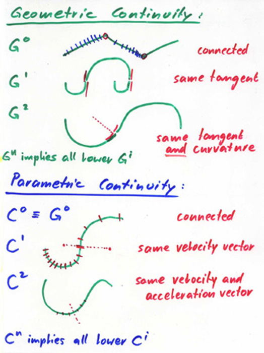
Warm-up: Geometric continuity versus Parametric continuity:
1.) Draw a closed curve that has G1 continuity (but not more), but does not have C1 continuity.
2.) Draw a closed curve that has C2 continuity, but does not have G1 continuity.
Lecture #13 -- Wed 3/7/2011.
Recall: Key concepts regarding Splines:
CG Splines are linearized approximations to natural splines that minimize bending energy.
A primary concern is with the
degrees
of smoothness of these curves:
-- Parametric Continuity: differentiability of the parametric
representation (C0, C1, C2, ...)
-- Geometric Continuity: smoothness of the resulting displayed
shape (G0=C0, G1=tangent-cont., G2=curvature-cont. )
Often we distinguish
between:
-- Interpolating splines (pass through all the data points;
example Hermite splines), and
-- Approximating splines (only come close to data points; example
B-Splines).
Another useful definition: the Turning Number of a curve
Remember the WINDING NUMBER of a closed curve around a given point: It specifies
how many times the position of a point moving along a curve circumnavigates the given point.
Now, the TURNING NUMBER of a curve specifies
how many rotations the direction of the tangent vector performs as it moves along the whole curve.
Cubic Bezier Curves
These very handy curves are a mixture of the above two "pure" schemes.
A Cubic Bezier Curve is defined by:
-- 2 interpolated endpoints, and
-- 2 approximated intermediary control points that define the tangent
directions at the endpoints.
Cubic polynomials: ==> allow to make inflection points and true space
curves in 3D.
Basic
underlying math;
(Cubic) Polynomial: infinitely differentiable --> Continuity = C-infinity
Cubic Hermite Spline: 2 endpoints, 2 tangent directions.
Cubic Bezier Curve: 2 endpoints, 2 approximated intermediary control
points.
-- (P1,P2) = 1/3 of starting velocity vector
-- (P3,P4) = 1/3 of ending velocity vector
Show influence of parameters (qualitative view).
Properties of Bezier Curves
Cubic polynomial, ==> true space curves;
Infinitely differentiable; (C-infinity)
May have loops, cusps; (only G0 is guaranteed)
Interpolates endpoints;
Approximation of the two central control points;
End tangents defined by pairs of control points;
Convex hull property; (curve lies completely inside the convex hull around its control polygon)
Variation diminishing; (straight line cannot cross curve more often than control polygon)
Invariant under affine transformations; (just need to transform the control points ...)
Start-to-end symmetry; (using control points in reverse order yields the same curve)
Construction of Bezier Curves
DeCasteljau
construction algorithm: (Construction by three iterations of linear
interpolation)
Show: The role of the control points.
-- How to draw a Bezier curve from its control points:
-- Subdivision of a Bezier curve into two pieces
that together are identical to the original one.
How
to put two Bezier segments together with G1 or with C1 continuity.
This is somewhat tedious! (More on curve constructions with Bezier segments next time)
Cubic B-Spline Curves
An easy way to make a smooth C2-continuous space curve (for the path of an
airplane or for a moving camera)
is to sprinkle a few control points through
space that define the coarse topology and geometry of the curve
and then
let them be approximated by a
cubic B-spline.
In a nutshell, one segment depending on the 4 control points A,B,C,D,
is given by the polynomial:
Q = A(1 -3t +3t2 -t3)/6 + B(4 -6t2 +3t3)/6 + C(1
+3t +3t2 -3t3)/6 + D(t3)/6
thus the point at t=0 is given by A/6 + 4B/6 + C/6,
and the point at t=1 is given by B/6 + 4C/6 + D/6.
Assuming for the moment a closed curve with N=6 control
points,
such a curve would be described as a sequence
of N=6 cubic curve segments,
each one of which is controlled by four
consecutive control points,
(but producing a curve segment that is only
about as long as the distance between the two middle control points.)
Because
a subsequent curve segment reuses three of the control points of the previous
segment,
they blend together in a very smooth (C2-continuous) way.
Properties of Cubic B-Splines
Piecewise cubic polynomial;
Does
NOT interpolate control points;
Convex hull property;
Variation diminishing;
Construction by 3-fold linear interpolation; (similar to the one for Bezier curves)
Invariant under affine transformations;
Start-to-end symmetry;
Twice differentiable (C2) at joints;
Infinitely differentiable everywhere else;
May have cusps, thus may not even be G1, everywhere;
Good to make smooth
closed loops (and roller-coaster tracks!).
DISCLAIMER: This is a very minimal introduction to cubic splines;
just enough to actually use them in As#7 and As#8.
[ More on splines in CS 284 and CS 283, CS 285 (These courses can be taken in any order). ]
Sweeps
To make a roller-coaster track, we use a generalized line-sweep:
A chosen cross-section of the track, which could be a simple rectangle,
is swept along a space curve (often called a "spine"),
while keeping one of its points (e.g., its centroid) on that spine.
The cross-sectional profile shape is always kept normal to the spine;
its rotation around the spine (azimuth) needs to be controlled procedurally or manually.
We start with a torsion-minimizing or rotation-minimizing frame (RMF),
and then use 3 control mechanisms to set the rotation angle everywhere along the spine:
-- a global, constant aximuth component: called azimuth;
-- a linealy varying azimuth component, starting at zero and building up to some total twist;
-- optional additional azimuth components specified at any of the spline control points,
which are interpolated with the same cubic polynomial as the x,y,z coordinates of the spine.
Discuss: What are reasonable azimuth specifications for a roller-coaster track?
Reading Assignments:
Shirley: [ 2nd Ed: 15.6-15.7 ]
Shirley: { 3rd Ed: 15.6-15.7 }
( Extract just enough so that you can get Assignments #7 and #8 done. )
Programming Assignment #7: May be done in pairs; due (electronically submitted) before Saturday 3/12, 11:00pm.
PREVIOUS
< - - - - > CS
184 HOME < - - - - > CURRENT
< - - - - > NEXT
Page Editor: Carlo
H. Séquin